1. Expected Values and Observed Values Usually Differ
 If I were to give you a coin and tell you to flip it 50 times, you’d expect the results to be about 50 heads and 50 tails. That’s a reasonable expectation, based on the fact that the coin has two sides, and your toss is a pretty good randomizer (assuming it’s an honest coin and that you make a vigorous toss: click here to read about how that isn’t always the case). But there’s a good chance that you won’t get 50/50. In four trials, you might observe:
- 48 heads and 52 tails.
- 45 heads and 55 tails
- 57 heads and 43 tails
- 60 heads and 40 tails
If the discrepancy is small (as in 48:52), it probably won’t bother you. You’ll say to yourself something like “This doesn’t bother me. It’s just random variation.” But there’s also a level at which the discrepancy becomes so great that it does bother you. You might start to wonder if something — another variable — is at play.
The difference between expected and observed results is a basic problem in the sciences. To solve this problem, scientists use a statistical method called the χ2 test. “χ” is the Greek letter “chi,” which (despite the “ch” at the start) is pronounced”kai” (and rhymes with “pie”). The test is pronounced “kai squared.”
Let’s see how it works.
2. Understanding the Null Hypothesis
Let’s start by getting some data from a genetic cross. We’ll use this to clarify some ideas related to the χ2 test, and then we’ll learn how to use the test.
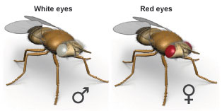
Here’s the scenario: a group of students is doing a breeding experiment with the fruit fly, Drosophila melanogaster. The students breed a white-eyed male (genotype XwY) with a red-eyed heterozygous female (genotype XWXw). Note that these are sex-linked genes alleles: click here for a review.
[qdeck]
[h] White-eyed male crossed with heterozygous red-eyed female
[q]1. Set up a Punnett square for a cross between a white-eyed male (genotype XwY) and a red-eyed heterozygous female, genotype XWXw
2. List the expected outcome for each phenotype.
[a]1. Here’s the Punnett square
| Xw | Y | |
| XW | XWXw | XWY |
| Xw | XwXw | XwY |
2. Here are the expected results:
1 red-eyed female: 1 white-eyed female: 1 red-eyed male: 1 white-eyed male.
[/qdeck]
The students’ experiment produced a total of 476 offspring. Based on the Punnett square, we’d expect four phenotypes, each equally represented. That means we expect 119 individuals of each type (divide 476 by 4 to get 119). The table below shows the observed results, and the expected results immediately below
| Red-Eyed Female | White-Eyed Female | Red-eyed male | White-eyed male | |
| Observed | 109 | 113 | 137 | 117 |
| Expected | 119 | 119 | 119 | 119 |
There’s a difference between the observed and expected results. We can respond in two ways.
- We can say, “We’re okay with this difference. The difference is insignificant, random, and not important. Our expectation (hypothesis) was correct.” Saying this means that we accept what statisticians call the NULL HYPOTHESIS. The null hypothesis means that there’s no statistically significant difference between observed and expected results.
- We can say “We’re not okay with this difference.” In that case, we do not accept the null hypothesis and have to conclude that
- Our expectation was flawed, or
- Our experimental methods were flawed.
What are the criteria by which we decide when to accept the null hypothesis, and when not to? That’s exactly what the χ2 test is for.
3. How to do a χ2 test in 7 steps
The formula for the χ2 test is
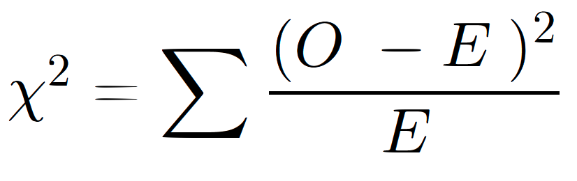
Here’s what each part of the equation means:
- χ2 is “chi-squared.” It’s what we’re solving for.
- Σ means “the sum of.”
- O means “observed.”
- E represents “expected.”
So, in plain English, the formula is
- χ2 equals the sum of ((observed – expected) squared), divided by the expected))
I’ve tried to use parentheses to show the order of operations. But if it’s not clear, it will be after we try it out.
To avoid confusion, I always do χ2 by setting up a table and then plugging in the numbers.
There are seven steps.
- STEP 1: Set up your table
- STEP 2: Enter the observed and expected values.
- STEP 3: In each column, subtract expected from observed: (O – E).
- STEP 4: In each column, square the value of observed – expected: (O-E)2
- STEP 5: In each column, divide (observed- expected)2 by the expected: (O-E)2/E.
- STEP 6: Add the values of (O-E)2/E.
- STEP 7: Look up the value in a critical values table (discussed below) and decide whether to accept your null hypothesis.
Let’s apply these steps to the problem above.
STEP 1: Set up your table. The number of rows is always the same. The number of columns varies based on the number of categories. In this case, there were four phenotypes, so we need four columns.
| Red-Eyed Female | White-Eyed Female | Red-eyed male | White-eyed male | |
| 1. Observed (O) | ||||
| 2. Expected (E) | ||||
| 3. Observed – Expected (O – E) | ||||
| 4. (O-E)2 | ||||
| 5. (O-E)2/E |
STEP 2: Enter the observed and expected values. Observed values are what you measured, tallied, etc. For the expected values, if you’re expecting equal representation, then just take the total and divide by the number of categories (as we’ll do here). If the expected ratios are not equal then you’d have to do a little more math to figure out your expected values. We’ll tackle that in the sample problems below.
| Red-Eyed Female | White-Eyed Female | Red-eyed male | White-eyed male | |
| 1. Observed (O) | 109 | 113 | 137 | 117 |
| 2. Expected (E) | 119 | 119 | 119 | 119 |
| 3. Observed – Expected (O – E) | ||||
| 4. (O-E)2 | ||||
| 5. (O-E)2/E |
STEP 3: Subtract expected from observed: (O – E). This is the value in row 1 – the value in row 2 in each column. Your answer can be a positive or a negative value.
| Red-Eyed Female | White-Eyed Female | Red-eyed male | White-eyed male | |
| 1. Observed (O) | 109 | 113 | 137 | 117 |
| 2. Expected (E) | 119 | 119 | 119 | 119 |
| 3. Observed – Expected (O – E) | -10 | -6 | 18 | -2 |
| 4. (O-E)2 | ||||
| 5. (O-E)2/E |
STEP 4: In each column, square the value of observed – expected: (O-E)2. This is the value in row 3 of each column, multiplied by itself.
| Red-Eyed Female | White-Eyed Female | Red-eyed male | White-eyed male | |
| 1. Observed (O) | 109 | 113 | 137 | 117 |
| 2. Expected (E) | 119 | 119 | 119 | 119 |
| 3. Observed – Expected (O – E) | -10 | -6 | 18 | -2 |
| 4. (O-E)2 | 100 | 36 | 324 | 4 |
| 5. (O-E)2/E |
STEP 5: In each column, divide (observed- expected)2 by the expected: (O-E)2/E. This is the value in row 4 divided by the value in row 2.
| Red-Eyed Female | White-Eyed Female | Red-eyed male | White-eyed male | |
| 1. Observed (O) | 109 | 113 | 137 | 117 |
| 2. Expected (E) | 119 | 119 | 119 | 119 |
| 3. Observed – Expected (O – E) | -10 | -6 | 18 | -2 |
| 4. (O-E)2 | 100 | 36 | 324 | 4 |
| 5. (O-E)2/E | 100/119=
0.84 |
36/119 =
0.30 |
324/119 =
2.72 |
4/119 =
0.03 |
STEP 6: Add the values of (O-E)2/E. These are all the values in row 5, added together.
0.84 + 0.13 + 2.72 + 0.03 = 3.89
So, for this data set χ2 = 3.89
STEP 7: Look up the value in a critical values table and decide whether or not to accept your null hypothesis.
The table below is a critical values table. Here’s how to use it.

-
- Determine the number of categories in your data set. In a genetics problem, that’s the number of phenotypes.
- Take the number of categories, and subtract 1. That’s your Degrees of Freedom (df)
- Find the table cell where probability (p-value) at the 0.05 level meets your degrees of freedom. Why 0.05? As someone who’s not a statistician (or even a scientist), I can only say that p = 0.05 is a widely agreed-upon standard for what constitutes statistical significance. As a student in an AP Bio course, that’s all you need to know. However, if you want to dig deeper into these issues, consult this page from the Statistics Teacher website.
- Determine if your χ2 value is less than the p = 0.05 value at the degrees of freedom for your problem.
- If it is less, then you ACCEPT the null hypothesis. That means that you interpret the difference between your observed and expected values as not being significant.
- If it isn’t less then you cannot accept the null hypothesis. You have to rethink your expectation or your experimental design.
Let’s apply these steps to the problem above.
- We have four categories (male with red eyes, male with white eyes, female with red eyes, and female with white eyes).
- Four categories – 1 = 3. That’s our degrees of freedom.
- The p-value for 0.05 meets 3 degrees of freedom at 7.82.
- Our χ2 was 3.89. Because 3.89 is less than 7.82, we accept our null hypothesis: the difference between observed and expected values was not statistically significant.
That’s it. Let’s make sure we’ve got the basic ideas, and then we’ll do some practice problems.
4. χ2: Checking Understanding
[qwiz qrecord_id=”sciencemusicvideosMeister1961-Chi Square Checking Understanding”] [h]
χ2: Key terms and Concepts
[q] χ2 is a statistical technique for evaluating the importance of the difference between [hangman] values (the ones that you measure) and [hangman] values.
[c]IG9ic2VydmVk[Qq]
[f]IENvcnJlY3Qh[Qq]
[c]IGV4cGVjdGVk[Qq]
[f]IEV4Y2VsbGVudCE=[Qq]
[q] The claim that the difference between observed and expected values is not statistically significant is known as the [hangman] [hangman].
[c]IG51bGw=[Qq]
[f]IEdvb2Qh[Qq]
[c]IGh5cG90aGVzaXM=[Qq]
[f]IEV4Y2VsbGVudCE=[Qq]
[q] An educator is studying the relationship between on-time attendance and grades. She divides the students who are the subject of a study into the following groups: early, on time, and tardy. After she gathers data and does her χ2 test, how many degrees of freedom will there be?
[textentry single_char=”true”]
[c]ID I=[Qq]
[f]IFllcy4gVGhlcmUgYXJlIHRocmVlIGNhdGVnb3JpZXMgYW5kIHR3byBkZWdyZWVzIG9mIGZyZWVkb20u[Qq]
[c]ICo=[Qq]
[f]IE5vLiBIZXJlJiM4MjE3O3MgYSBoaW50LiBUaGUgZGVncmVlcyBvZiBmcmVlZG9tIGlzIHRoZSBudW1iZXIgb2YgY2F0ZWdvcmllcyAtMS4gSG93IG1hbnkgY2F0ZWdvcmllcyBhcmUgdGhlcmU/[Qq]
[q] In peas, the allele for purple flowers (P) is dominant over the allele for white flowers (p). If you carry out a monohybrid cross, and then statistically analyze the results using a χ2 test, how many degrees of freedom will there be?
[textentry single_char=”true”]
[c]ID E=[Qq]
[f]IFllcy4gVGhlcmUgYXJlIG9ubHkgdHdvIHBoZW5vdHlwZSBjYXRlZ29yaWVzLCBwdXJwbGUgYW5kIHdoaXRlLCBzbyB0aGUgZGVncmVlcyBvZiBmcmVlZG9tID0gMS4=[Qq]
[c]ICo=[Qq]
[f]IE5vLiBIZXJlJiM4MjE3O3MgdGhlIG1vbm9oeWJyaWQgY3Jvc3M6
Cg==| [Qq] | P | p |
| P | PP | Pp |
| p | Pp | pp |
P is dominant. How many phenotypic categories will there be? Take that number, subtract 1, and you’ll have the degrees of freedom.
[q multiple_choice=”true”] A student is evaluating the phenotypic results of a dihybrid cross: AaBb x AaBb. If they want to evaluate their phenotypic results at the 0.05 probability level, what critical value do they use?
[c]IDMuODQ=[Qq]
[f]IE5vLiBBIGRpaHlicmlkIGNyb3NzIHdpbGwgcmVzdWx0IGluIGZvdXIgcGhlbm90eXBpYyBjYXRlZ29yaWVzOg==
Cg==- Cg==
- RG9taW5hbnQgZm9yIGJvdGggdHJhaXRzOw== Cg==
- [Qq]Dominant for the first trait, recessive for the second;
- Recessive for the first trait, dominant for the second;
- Recessive for both traits.
The number of degrees of freedom is the number of categories – 1. Find where the p-value of 0.05 intersects with that many degrees of freedom, and you’ll have the answer.
[c]IDUuOTk=[Qq]
[f]IE5vLiBBIGRpaHlicmlkIGNyb3NzIHdpbGwgcmVzdWx0IGluIGZvdXIgcGhlbm90eXBpYyBjYXRlZ29yaWVzOg==
Cg==- Cg==
- RG9taW5hbnQgZm9yIGJvdGggdHJhaXRzOw== Cg==
- [Qq]Dominant for the first trait, recessive for the second;
- Recessive for the first trait, dominant for the second;
- Recessive for both traits.
The number of degrees of freedom is the number of categories – 1. Find where the p-value of 0.05 intersects with that many degrees of freedom, and you’ll have the answer.
[c]IDcu ODI=[Qq]
[f]IEV4Y2VsbGVudC4gQSBkaWh5YnJpZCBjcm9zcyB3aWxsIHJlc3VsdCBpbiBmb3VyIHBoZW5vdHlwaWMgY2F0ZWdvcmllczo=
Cg==- Cg==
- RG9taW5hbnQgZm9yIGJvdGggdHJhaXRzOw== Cg==
- [Qq]Dominant for the first trait, recessive for the second;
- Recessive for the first trait, dominant for the second;
- Recessive for both traits.
The number of degrees of freedom is the number of categories – 1. In this case, it’s 4 categories, so 3 degrees of freedom. The p-value of 0.05 intersects with 3 degrees of freedom at 7.82.
[c]IDkuNDk=[Qq]
[f]IE5vLiBBIGRpaHlicmlkIGNyb3NzIHdpbGwgcmVzdWx0IGluIGZvdXIgcGhlbm90eXBpYyBjYXRlZ29yaWVzOg==
Cg==- Cg==
- RG9taW5hbnQgZm9yIGJvdGggdHJhaXRzOw== Cg==
- [Qq]Dominant for the first trait, recessive for the second;
- Recessive for the first trait, dominant for the second;
- Recessive for both traits.
The number of degrees of freedom is the number of categories – 1. Find where the p-value of 0.05 intersects with that many degrees of freedom, and you’ll have the answer.
[q multiple_choice=”true”] A student is evaluating the phenotypic results of a test cross: AABb x aabb. If they want to evaluate their data at the 0.05 probability level, what critical value do they use?
[c]IDMu ODQ=[Qq]
[f]IE5pY2Ugam9iLiBUaGUgdGVzdCBjcm9zcyBiZXR3ZWVuIEFBQmIgYW5kIGFhYmIgcmVzdWx0cyBpbiB0d28gZ2Vub3R5cGVzIGFuZCB0d28gcGhlbm90eXBlczo=
Cg==- Cg==
- QWFCYjogRG9taW5hbnQgZm9yIGJvdGggdHJhaXRzOw== Cg==
- [Qq]Aabb: Dominant for the first trait, recessive for the second trait.
The number of degrees of freedom is the number of categories – 1. That’s one degree of freedom. The p-value of 0.05 intersects with one degree of freedom at 3.84.
[c]IDUuOTk=[Qq]
[f]IE5vLiBUaGUgdGVzdCBjcm9zcyBiZXR3ZWVuIEFBQmIgYW5kIGFhYmIgcmVzdWx0cyBpbiB0d28gZ2Vub3R5cGVzIGFuZCB0d28gcGhlbm90eXBlczo=
Cg==- Cg==
- QWFCYjogRG9taW5hbnQgZm9yIGJvdGggdHJhaXRzOw== Cg==
- [Qq]Aabb: Dominant for the first trait, recessive for the second trait.
The number of degrees of freedom is the number of categories – 1. Find where the p-value of 0.05 intersects with that many degrees of freedom, and you’ll have the answer.
[c]IDcuODI=[Qq]
[f]IE5vLlRoZSB0ZXN0IGNyb3NzIGJldHdlZW4gQUFCYiBhbmQgYWFiYiByZXN1bHRzIGluIHR3byBnZW5vdHlwZXMgYW5kIHR3byBwaGVub3R5cGVzOg==
Cg==- Cg==
- QWFCYjogRG9taW5hbnQgZm9yIGJvdGggdHJhaXRzOw== Cg==
- [Qq]Aabb: Dominant for the first trait, recessive for the second trait.
The number of degrees of freedom is the number of categories – 1. Find where the p-value of 0.05 intersects with that many degrees of freedom, and you’ll have the answer.
[c]IDkuNDk=[Qq]
[f]IE5vLlRoZSB0ZXN0IGNyb3NzIGJldHdlZW4gQUFCYiBhbmQgYWFiYiByZXN1bHRzIGluIHR3byBnZW5vdHlwZXMgYW5kIHR3byBwaGVub3R5cGVzOg==
Cg==- Cg==
- QWFCYjogRG9taW5hbnQgZm9yIGJvdGggdHJhaXRzOw== Cg==
- [Qq]Aabb: Dominant for the first trait, recessive for the second trait.
The number of degrees of freedom is the number of categories – 1. Find where the p-value of 0.05 intersects with that many degrees of freedom, and you’ll have the answer.
[q multiple_choice=”true”] In incomplete dominance, heterozygotes have an intermediate phenotype. A scientist is performing a statistical analysis of the outcome of a monohybrid cross for a trait that involves incomplete dominance. If they want to evaluate their data at the 0.05 probability level, what critical value do they use?
[c]IDMuODQ=[Qq]
[f]IE5vLiBJbiBpbmNvbXBsZXRlIGRvbWluYW5jZSwgYSBtb25vaHlicmlkIGNyb3NzIChzdWNoIGFzIHRoYXQgYmV0d2VlbiBBYSBhbmQgQWEpIHdpbGwgcmVzdWx0IGluIHRocmVlIHBoZW5vdHlwZXM6
Cg==- Cg==
- QUE6IERvbWluYW50IHBoZW5vdHlwZQ== Cg==
- [Qq]Aa: Intermediate phenotype
- aa: Recessive phenotype
The number of degrees of freedom is the number of categories – 1. Find where the p-value of 0.05 intersects with that many degrees of freedom, and you’ll have the answer.
[c]IDUu OTk=[Qq]
[f]IE5pY2Ugam9iISBJbiBpbmNvbXBsZXRlIGRvbWluYW5jZSwgYSBtb25vaHlicmlkIGNyb3NzIChzdWNoIGFzIHRoYXQgYmV0d2VlbiBBYSBhbmQgQWEpIHdpbGwgcmVzdWx0IGluIHRocmVlIHBoZW5vdHlwZXM6
Cg==- Cg==
- QUE6IERvbWluYW50IHBoZW5vdHlwZQ== Cg==
- [Qq]Aa: Intermediate phenotype
- aa: Recessive phenotype
The number of degrees of freedom is the number of categories – 1. In this case, 3 phenotypes means 2 degrees of freedom. The p-value of 0.05 intersects with that many degrees of freedom at 5.99.
[c]IDcuODI=[Qq]
[f]IE5vLiBJbiBpbmNvbXBsZXRlIGRvbWluYW5jZSwgYSBtb25vaHlicmlkIGNyb3NzIChzdWNoIGFzIHRoYXQgYmV0d2VlbiBBYSBhbmQgQWEpIHdpbGwgcmVzdWx0IGluIHRocmVlIHBoZW5vdHlwZXM6
Cg==- Cg==
- QUE6IERvbWluYW50IHBoZW5vdHlwZQ== Cg==
- [Qq]Aa: Intermediate phenotype
- aa: Recessive phenotype
The number of degrees of freedom is the number of categories – 1. Find where the p-value of 0.05 intersects with that many degrees of freedom, and you’ll have the answer.
[c]IDkuNDk=[Qq]
[f]IE5vLiBJbiBpbmNvbXBsZXRlIGRvbWluYW5jZSwgYSBtb25vaHlicmlkIGNyb3NzIChzdWNoIGFzIHRoYXQgYmV0d2VlbiBBYSBhbmQgQWEpIHdpbGwgcmVzdWx0IGluIHRocmVlIHBoZW5vdHlwZXM6
Cg==- Cg==
- QUE6IERvbWluYW50IHBoZW5vdHlwZQ== Cg==
- [Qq]Aa: Intermediate phenotype
- aa: Recessive phenotype
The number of degrees of freedom is the number of categories – 1. Find where the p-value of 0.05 intersects with that many degrees of freedom, and you’ll have the answer.
[/qwiz]
5. χ2 Practice Problems
At this point, you should be ready for some practice problems. Set up your data in tables, systematically follow the seven steps I laid out above, and you’ll be fine.
[qdeck scroll = “true” style=” min-height: 600px !important; width: 675px !important;” card_back=”none” qrecord_id=”sciencemusicvideosMeister1961-Chi Square Practice Problems”]
[h] χ2 Practice Problems
[q] In corn, purple seeds are dominant over yellow seeds. Smooth seeds are dominant to wrinkled. In an experimental dihybrid cross, the following results were obtained.
| Phenotype | Purple Smooth | Purple Wrinkled | Yellow Smooth | Yellow Wrinkled |
| Observed | 190 | 60 | 79 | 18 |
Run a χ2 test to determine if the difference between observed and expected is significant or not. Your answer 1) will list a χ2 value, 2) interpret the results in a way that accepts or fails to accept the null hypothesis, with a justification of your interpretation.
[a] Because this is a dihybrid cross, you’re expecting a 9:3:3:1 ratio. Of the 347 offspring, that means that you expect 9/16 to have both dominant traits. So, multiply 347 by 9/16, and you have 195.19 that you’re expecting with that phenotype. Determine your other expected numbers by multiplying the total by 3/16 and 1/16.
| Purple, smooth | Purple wrinkled | yellow, smooth | yellow, wrinkled | total | |
| observed | 190 | 60 | 79 | 18 | 347 |
| expected | 195.2 | 65.1 | 65.1 | 21.7 | |
| o-e | -5.2 | -5.1 | 13.9 | -3.7 | |
| (o-e)(o-e) | 26.9 | 25.6 | 194.3 | 13.6 | |
| ((o-e)(o-e))/e | 0.14 | 0.39 | 2.99 | 0.63 | 4.14 |
The χ2 value is 4.14. There are 4 categories, meaning 3 degrees of freedom, so the critical value at the 0.05 level is 7.82. Because 4.14 is below 7.82, we can accept the null hypothesis. The difference is not statistically significant.
[q] In Drosophila, the white-eyed trait is a recessive, sex-linked mutation. In a breeding experiment, a white-eyed male is crossed with a heterozygous, red-eyed female. The following results were obtained:
| phenotype | male, white eyes | male, normal eyes | female, white eyes | female, normal eyes |
| observed | 86 | 109 | 115 | 133 |
Run a χ2 test to determine if the difference between observed and expected is significant or not. Your answer 1) will list a χ2 value, 2) interpret the results in a way that accepts or fails to accept the null hypothesis, with a justification of your interpretation.
[a] If you make this Punnett square…
| Xw | Y | |
| XW | XWXw | XWY |
| Xw | XwXw | XwY |
Running a χ2 test on the data above gives you the following:
| phenotype | male, white eyes | male, normal eyes | female, white eyes | female, normal eyes | total |
| observed | 86 | 109 | 115 | 133 | 443 |
| expected | 110.8 | 110.8 | 110.8 | 110.8 | |
| o-e | -24.8 | -1.8 | 4.3 | 22.3 | |
| (o-e)(o-e) | 612.6 | 3.1 | 18.1 | 495.1 | |
| (o-e)(o-e)/e | 5.5 | 0.0 | 0.2 | 4.5 | 10.2 |
χ2 = 10.2. There are 4 categories, meaning 3 degrees of freedom, so the critical value at the 0.05 level is 7.82. Because 10.2 is above 7.82, we cannot accept the null hypothesis. The difference is statistically significant, and (since we know that our hypothesis is correct), we need to look for additional variables that are causing the discrepancy.
[q] In Drosophila, apterous is a mutation that causes flies to develop extremely reduced or absent wings. The mutation is autosomal and recessive. Two flies, both heterozygous normal, are bred together, with the following results.
| Phenotype | Normal wings | apterous |
| Observed | 643 | 189 |
- Using the symbols ap+ and vg, create a Punnett square and make a hypothesis about expected results.
- Run a χ2 test to determine if the difference between observed and expected is significant or not. Your answer 1) will list a χ2 value, 2) interpret the results in a way that accepts or fails to accept the null hypothesis, with a justification of your interpretation.
[a] 1. If you make this Punnett square…
| ap+ | ap | |
| ap+ | ap+ ap+ | ap+ ap |
| ap | ap+ ap | ap ap |
…you’d expect 3/4 normal winged, and 1/4 apterous
That leads to the following χ2 test on the data above gives you the following:
| male, normal wings | female, apterous | total | |
| observed | 643 | 189 | 832 |
| expected | 624.0 | 208.0 | |
| o-e | 19.0 | -19.0 | |
| (o-e)(o-e) | 361.0 | 361.0 | |
| (o-e)(o-e)/e | 0.6 | 1.7 | 2.3 |
The χ2 value is 2.3. There are 2 categories, meaning 1 degree of freedom, so the critical value at the 0.05 level is 3.84. Because 2.3 is below 3.84, we can accept the null hypothesis. The difference is not statistically significant.
[q] In Drosophila, sepia (se) is a mutation that produces brown eyes. This allele is autosomal and recessive to the wild-type allele (se+), which produces red eyes. Apterous (ap) is an autosomal recessive mutation resulting in reduced or absent wings. The wild-type allele is ap+).
Students in a lab perform a dihybrid cross. In addition to looking at the phenotypes for sepia and apterous, they also categorize their flies by sex. Here are their results.
| male, normal wing, normal eye | female, normal wing, normal eye | male, apterous, normal eye | female, apterous, normal eye | male, normal wing, sepia eyes | female, normal wing, sepia eyes | male, apterous, sepia | female, apterous, sepia | |
| observed | 196 | 358 | 57 | 90 | 85 | 117 | 16 | 21 |
- Make a hypothesis about expected results.
- Run a χ2 test to determine if the difference between observed and expected is significant or not. Your answer 1) will list a χ2 value, 2) interpret the results in a way that accepts or fails to accept the null hypothesis, with a justification of your interpretation.
[a] 1. This is a dihybrid cross, so you’re expecting a 9:3:3:1 ratio. But adding sex, you’re expecting 9/32 male wild type, 9/32 female wild type, 3/32 male normal wings, sepia eyes, 3/32 female normal wings sepia eyes, etc.
2. Your χ2 test is as follows:
| male, normal wing, normal eye | female, normal wing, normal eye | male, apterous, normal eye | female, apterous, normal eye | male, normal wing, sepia eyes | female, normal wing, sepia eyes | male, apterous, sepia | female, apterous, sepia | total | |
| observed | 196 | 358 | 57 | 90 | 85 | 117 | 16 | 21 | 940 |
| expected | 264.4 | 264.4 | 88.1 | 88.1 | 88.1 | 88.1 | 29.4 | 29.4 | |
| o-e | -68.4 | 93.6 | -31.1 | 1.9 | -3.1 | 28.9 | -13.4 | -8.4 | |
| (o-e)(o-e) | 4675.1 | 8765.6 | 968.8 | 3.5 | 9.8 | 833.8 | 178.9 | 70.1 | |
| (o-e)(o-e)/e | 17.7 | 33.2 | 11.0 | 0.0 | 0.1 | 9.5 | 6.1 | 2.4 | 79.9 |
χ2 = 79.9. There are 8 categories, meaning 7 degrees of freedom, so the critical value at the 0.05 level is 15.51. Because 79.9 is above 15.51, we cannot accept the null hypothesis. The difference is statistically significant, and (since we know that our hypothesis is correct), we need to look for additional variables that are causing the discrepancy.
[/qdeck]
What now?
- Continue to Mitochondrial Inheritance, Incomplete Dominance, and Genotype-Environment Interaction (the last tutorial in this module)
- Return to the Genetics Main Menu