1. Introduction to Population Ecology
In biology, a population is defined as a group of organisms of the same species inhabiting a particular location.
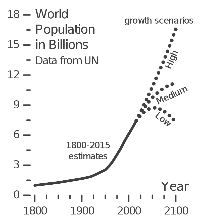 The diagram to your left, which uses data from the United Nations, shows how the size of humanity’s population has changed over the past two hundred years. The Earth’s human population was about one billion in 1800. In 1961 (when Mr. W. was born), it was three billion. Now, it’s about 7.5 billion.
What about the future? It depends on a variety of factors, especially birth rate (the number of births/year). The low projection sees the human population reaching a maximum size in about 2040, then starting to decline. Why? because in many parts of the world, birth rates are falling. The medium projection sees population growth continuing, but at a slower rate. And the high scenario sees the current rate continuing.
As human populations have grown, populations of wildlife have fallen. These numbers are less precise, but it’s thought that there were about 12 million African elephants in the early 1900s. Now there are about 350,000 (source: Africa Geographic).
2. How Populations Grow
To learn how populations grow, complete the interactive reading below.
[qwiz qrecord_id=”sciencemusicvideosmeister1961-Population Growth, Interactive Reading (v2.0)”]
[h]Population growth: interactive reading
[i]
[q labels = “top”] Think of the city or town where you live. On the most fundamental level, only four events will determine whether your town or city’s population goes up or goes down. Think about what these are and complete what’s below.
- Things that increase population: _________ and _____________ (movement into a population).
- Things that decrease population: _________ and _____________ (movement out of a population.
[l]birth
[fx] No. Please try again.
[f*] Excellent!
[l]death
[fx] No. Please try again.
[f*] Excellent!
[l]immigration
[fx] No, that’s not correct. Please try again.
[f*] Great!
[l]emigration
[fx] No. Please try again.
[f*] Correct!
[q labels = “top”]To simplify what’s going to come, we’re going to assume that immigration and emigration are equal. With that assumed, then the growth rate (the change in population over time) can be expressed as follows
________ rate = birth rate – _________ rate
or, with symbols
r = __ – d
[l]death
[fx] No. Please try again.
[f*] Great!
[l]growth
[fx] No. Please try again.
[f*] Correct!
[l]b
[fx] No, that’s not correct. Please try again.
[f*] Good!
[q]Just to review:
r = b – d
means
growth rate = [hangman] rate – [hangman] rate.
That means, of course, that population only grows if [hangman] rate is greater than the [hangman] rate. If the reverse is true, the population will [hangman].
[c]YmlydGg=[Qq]
[c]ZGVhdGg=[Qq]
[c]YmlydGg=[Qq]
[c]ZGVhdGg=[Qq]
[c]ZGVjcmVhc2U=[Qq]
[q]Another way to express this is to think about the change in a population’s size over time. This is typically expressed by the following formula.
dN/dt=rN
where
- dN means “the change in population”
- dt means “the change in time”
- r is the “growth rate”
- N is the population
In this formula, if r > 1, then the population will _________. If r < 1, then the population will __________.
[l]decrease
[fx] No. Please try again.
[f*] Great!
[l]grow
[fx] No. Please try again.
[f*] Great!
[q]To connect this to something that might be more familiar, just think about money. If you put $100 into a bank account that paid 2% yearly interest, how much money would you have at the end of the year? Note that I’m using “$” to indicate a quantity of money.
Start by converting 2% to 1.02
Then use the formula d$/dt=r$
Your change in value would be calculated as
d$/dt=1.02(100)
d$/dt=$102
[q]Populations will grow in the same way as money in the bank will. The key point is that each year’s ending point becomes the next year’s starting point. So if your interest rate were 3%, and your initial investment was $1000, your money would grow as follows.
Note that each year, your money grows a bit more. By year 14 you’re adding $44/year, compared to year 1, when you added only $30. The result is what’s called exponential growth.
[/qwiz]
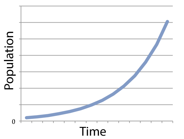
If you graph a system (like a population) that’s growing exponentially, you get something that looks like what’s shown on the left.
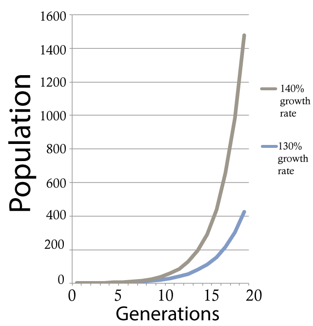 Note that it doesn’t matter if your rate of growth is 0.03% or 5%: any growth rate will lead to exponential growth, as long as the growth rate is constant over time. The only difference is how long it’ll take before the line starts to steeply shoot upward. For example, the gray line on the right shows growth at 40 %/year. The blue line shows 30 %/year. Notice how in both cases, there’s a long takeoff period. Many generations have to go by before the lines start to rise upward to any appreciable degree. Think of that takeoff as being similar to the time an airplane spends moving down the runway until it’s moving quickly enough to take off. The higher the growth rate, the less time is required on the runway.
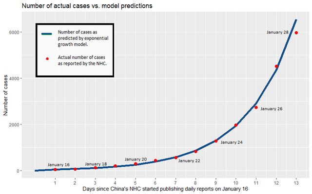
Here’s another example of exponential growth. This one relates to the very start of the COVID-19 pandemic. The graph below shows cases of COVID-19 over two weeks in China from January 10 to January 24, 2020. Take a look at the legend, and note how closely the number of reported cases matches the number of cases predicted by the exponential growth model.
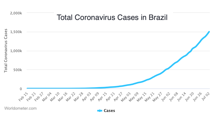
In countries where effective public health measures were not implemented, COVID-19 continued to spread at an exponential rate. Here’s a graph of how the pandemic unfolded in Brazil between February and June of 2020. Click on the image to enlarge it. Note how the time scale and the number of cases differ from the graph of China’s experience, but that the shape of the line is the same.
Biotic potential is “the ability of a population …. to increase under ideal environmental conditions — sufficient food supply, no predators, and a lack of disease. An organism’s rate of reproduction and the size of each litter are the primary determining factors for biotic potential.” (source: populationeducation.org).
Biotic potential is represented as rmax. When nothing impedes rmax, populations grow exponentially.
3. Carrying Capacity, Limiting Factors, and Logistic Growth
In any finite system — including Planet Earth — exponential growth can’t go on forever. Eventually, a growing population reaches the environment’s carrying capacity. Complete the interactive reading below to see how carrying capacity works.
[qwiz style=”width: 730px !important; min-height: 450px !important;” qrecord_id=”sciencemusicvideosMeister1961-Carrying Capacity and Logistic Growth: Interactive Reading (v2.0)”]
[h] Carrying Capacity and Logistic Growth: Interactive Reading
[q labels = “top”] Carrying capacity is the maximum number of individuals of a particular species that a specific environment can support. It’s represented by the letter K. As a population’s size (N) approaches K, then population growth _______________. Why? Either b ___________ or d ___________ (or both).
[l] decreases
[f*] Good!
[fx] No. Please try again.
[l] increases
[f*] Correct!
[fx] No, that’s not correct. Please try again.
[l]slows down
[f*] Excellent!
[fx] No, that’s not correct. Please try again.
[q labels = “top”] Here’s the formula for logistic growth. Translate it into words by dragging in the correct terms
[f*] Good!
[fx] No, that’s not correct. Please try again.
[l]carrying capacity
[f*] Excellent!
[fx] No. Please try again.
[l]population
[f*] Correct!
[fx] No. Please try again.
[l]time
[f*] Good!
[fx] No. Please try again.
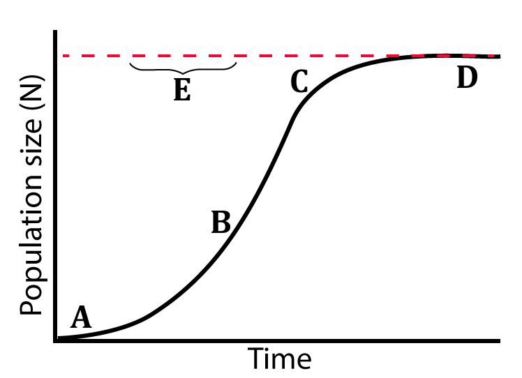
[q] In the diagram at left, the dotted line at “E” represents the carrying capacity. Carrying capacity is a function of limiting factors. Imagine a small population of deer that swim to a large island that lacks both deer and predators, but has plenty of grass and shrubs. Without any limits, the deer grow at their rmax. The growth is slow at first. This initial phase (shown at A) is called a lag phase.
After the lag phase, growth accelerates ( shown at B). During this period the growth is similar to what you’d see in a population that’s growing exponentially. Accordingly, “B” is called the exponential growth phase.
At a certain point, the deer population grows to a point where there begins to be a significant amount of competition for food. Food scarcity starts to limit population growth. At “C” you can see population growth starting to level off. This is often referred to as a “deceleration phase.” At “D,” the population has reached its carrying capacity.
[q] In the diagram below, which number represents the carrying capacity?
[textentry single_char=”true”]
[c]IE U=[Qq]
[f]IEV4Y2VsbGVudC4gJiM4MjIwO0UmIzgyMjE7IHJlcHJlc2VudHMgY2FycnlpbmcgY2FwYWNpdHk=[Qq]
[c]ICo=[Qq]
[f]IE5vLiBZb3UmIzgyMTc7cmUgbG9va2luZyBmb3IgYSBsaW5lIHRoYXQgcmVwcmVzZW50cyB0aGUgbWF4aW11bSBwb3B1bGF0aW9uIHRoYXQgdGhpcyBhcmVhIG9yIGVudmlyb25tZW50IGNvdWxkIHN1cHBvcnQu[Qq]
[q] In the diagram below, which letter represents the point at which the population is growing the fastest?
[textentry single_char=”true”]
[c]IE I=[Qq]
[f]IE5pY2Ugam9iLiAmIzgyMjA7QiYjODIyMTsgaXMgdGhlIHBvaW50IGF0IHdoaWNoIHRoaXMgcG9wdWxhdGlvbiBpcyBpbmNyZWFzaW5nIHRoZSBmYXN0ZXN0Lg==[Qq]
[c]ICo=[Qq]
[f]IE5vLiBMb29rIGZvciB0aGUgcG9pbnQgaW4gdGhlIGJsYWNrIGxpbmUgd2hlcmUgdGhlIHNsb3BlIGlzIHRoZSBzdGVlcGVzdC4=[Qq]
[q] In the diagram below, which letter represents the point at which the population has reached the environment’s carrying capacity?
[textentry single_char=”true”]
[c]IE Q=[Qq]
[f]IEF3ZXNvbWUuICYjODIyMDtEJiM4MjIxOyBpcyB0aGUgcG9pbnQgYXQgd2hpY2ggdGhpcyBwb3B1bGF0aW9uIGhhcyByZWFjaGVkIGl0cyBjYXJyeWluZyBjYXBhY2l0eS4=[Qq]
[c]ICo=[Qq]
[f]IE5vLiBMb29rIGZvciB0aGUgcG9pbnQgaW4gdGhlIGJsYWNrIGxpbmUgd2hlcmUgdGhlIHNsb3BlIGlzIHRoZSBzdGVlcGVzdC4=[Qq]
[q] Pretend that the population represented below had feelings. Which letter represents the point at which the population would start to feel resistance to its exponential growth?
[textentry single_char=”true”]
[c]IE M=[Qq]
[f]IEdvb2Qgam9iLiAmIzgyMjA7QyYjODIyMTsgaXMgdGhlIHBvaW50IGF0IHdoaWNoIHRoaXMgcG9wdWxhdGlvbiB3b3VsZCBzdGFydCB0byBmZWVsIHJlc2lzdGFuY2UgZnJvbSB0aGUgZW52aXJvbm1lbnQuIFRoYXQmIzgyMTc7cyB0aGUgcG9pbnQgd2hlcmUgaXQmIzgyMTc7cyBhcHByb2FjaGluZyBpdHMgY2FycnlpbmcgY2FwYWNpdHku[Qq]
[c]ICo=[Qq]
[f]IE5vLiBMb29rIGZvciB0aGUgcG9pbnQgaW4gdGhlIGJsYWNrIGxpbmUgd2hlcmUgdGhlIGxpbmUgaXMgc3RhcnRpbmcgdG8gc2xvcGUgbGVzcyBzdGVlcGx5IHVwd2FyZC4gVGhhdCBkZWNyZWFzZWQgc2xvcGUgaXMgZnJvbSByZXNpc3RhbmNlIGZyb20gdGhlIGVudmlyb25tZW50LCBjYXVzaW5nIGVpdGhlciBhIGRlY3JlYXNlIGluIHRoZSBiaXJ0aCByYXRlIG9yIGFuIGluY3JlYXNlIGluIHRoZSBkZWF0aCByYXRlLiBXaGVyZSBvbiB0aGUgYmxhY2sgbGluZSBkb2VzIHRoZSBzbG9wZSBzdGFydCB0byBkZWNyZWFzZT8=[Qq]
[q] In the diagram below, which letter represents the lag phase?
[textentry single_char=”true”]
[c]IE E=[Qq]
[f]IEV4Y2VsbGVudC4gJiM4MjIwO0EmIzgyMjE7IGlzIHRoZSBsYWcgcGhhc2UsIGEgcGVyaW9kIG9mIHZlcnkgc2xvdyBncm93dGggdGhhdCBvY2N1cnMgd2hlbiBhIHBvcHVsYXRpb24gaXMganVzdCBnZXR0aW5nIHN0YXJ0ZWQu[Qq]
[c]ICo=[Qq]
[f]IE5vLiBJbWFnaW5lIHRoYXQgdGhlIHBvcHVsYXRpb24gd2FzIGFuIGFpcnBsYW5lLiBCZWZvcmUgaXQgdGFrZXMgb2ZmLCBpdCBoYXMgdG8gbW92ZSBkb3duIHRoZSBydW53YXkgYW5kIHBpY2sgdXAgc3BlZWQuIFdoaWNoIGxldHRlciB3b3VsZCBiZXN0IHJlcHJlc2VudCB0aGUgcnVud2F5IGJlZm9yZSB0YWtlb2ZmPw==[Qq]
[/qwiz]
4. Density-Dependent and Density-Independent Limiting Factors
The two models of population growth described above have a variety of terms connected to them. Take a minute to study the table below.
| Graph | |
 |
| Graph description | J Curve | S Curve, Sigmoid Curve |
| Growth Model | Exponential Growth | Logistic Growth |
Carrying capacity, a key part of the logistic growth model, can be thought of as environmental resistance. As a population grows toward the environment’s carrying capacity, various factors in the environment start to limit a population’s capacity for continued growth. These are called limiting factors, and they fall into two categories.
Density-dependent limiting factors become more intense as the density of a population increases. For example, as a population’s density increases,
- There’s more competition for food, shelter, mates, etc.
- It becomes easier for parasites to spread from one individual to the next.
- If the members of this population are potential prey for another species, then predation might increase.
- Wastes can accumulate, fouling the environment (which can then become more conducive to parasites).
All of the factors listed above are classified as extrinsic factors: that’s because they come from outside the population. Other density-dependent limiting factors are intrinsic. For example, increased crowding might cause stress, which leads to a decrease in the birth rate.
Density-independent limiting factors aren’t a function of increased population density. Consider a population of anole lizards on an island in the Caribbean. A hurricane strikes the island, completely swamping it with a tidal surge. Whether the lizard’s population is large or small, this storm will kill many, if not all of the lizards. The same could be said of almost any natural disaster.
5. What happens as populations approach K?
The logistic growth model is a mathematical model. In nature or experimental studies with actual organisms, a variety of things can happen as a population approaches the environment’s carrying capacity.
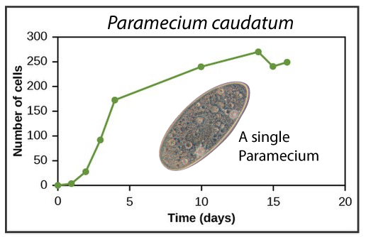
In the 1930s, Russian biologist Georgy Gause studied the growth rates of Paramecia, a single-celled, ciliated eukaryote. In two separate species (only one of which is shown at left), the pattern of growth roughly followed the logistic growth model.
Here’s a different representation of what happens as a population reaches its carrying capacity.
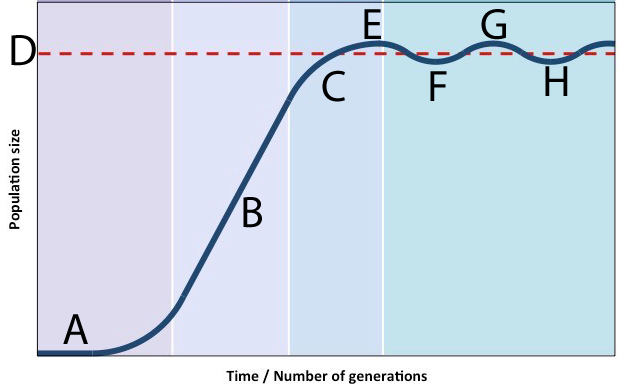
In this scenario, the population’s growth decelerates (C) as it approaches carrying capacity. The peak population that’s reached (E) is actually above the carrying capacity (D). Consumption of resources beyond carrying capacity degrades the environment and depletes available resources. This lowers carrying capacity. As a result, the population falls (as shown at F). With the population at this level, the environment recovers, allowing the population to grow. What we have, in other words, is a stable oscillation around carrying capacity.
Here’s another scenario:
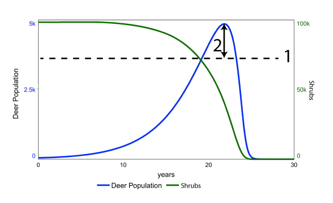
Think back to the small group of deer who swim to an island with abundant vegetation and no predators. The blue line shows the subsequent growth of the deer population. In this case, the population grows significantly beyond the island’s initial carrying capacity (at “1”). This is called an overshoot, and it’s indicated by the double-headed arrow at “2.”
The overshoot causes significant depletion of the island’s resource base. As the population of shrubs diminishes, so does the population of deer. By the end of the process, the vegetation is gone, and the island’s deer have become locally extinct.
Interactions between predators and their prey can result in population oscillations, as shown in the graph below.
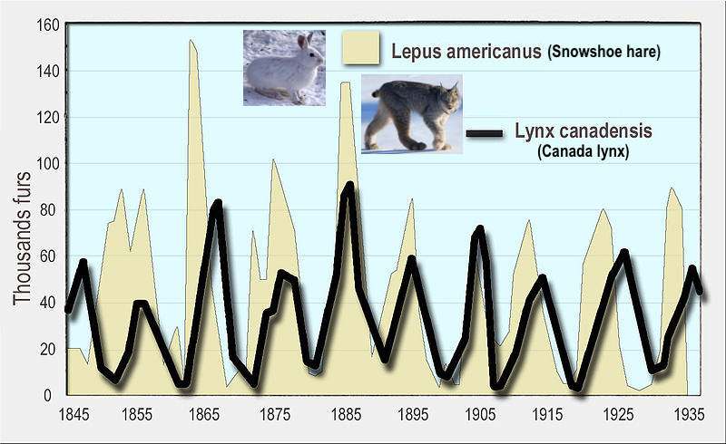
The Canada Lynx (Lynx canadensis) is a medium-sized cat that’s about twice the size of a house cat. It’s adapted for life in Canada and Alaska. The lynx’s primary prey is the snowshoe hare (Lepus americanus).
The data in this graph is based on pelts collected by trappers and sold to the Hudson Bay Company for about 100 years.
While this looks like density-dependent regulation of the hare’s population by the lynx, the interaction is more complex. Read the lightly edited passage below from Wikipedia:
A specialist predator, the Canada lynx depends heavily on snowshoe hares for food. Snowshoe hare populations in Alaska and central Canada undergo cyclic rises and falls—at times the population densities can fall from as high as 2,300/km2 (6,000/sq. mi) to as low as 12/km2 (31/sq. mi). Consequently, a period of hare scarcity occurs every 8 to 11 years. An example of a prey-predator cycle, the cyclic variations in snowshoe hare populations significantly affect the numbers of their predators—lynxes and coyotes—in the region. When the hare populations plummet, lynxes tend to move to areas with more hares and tend to not produce litters.
In northern Canada, the abundance of lynx can be estimated from the records kept of the number caught each year for their fur; records have been kept by the Hudson’s Bay Company and the Canadian government since the 1730s. These cycles…are caused by the interplay of three major factors—food, predation, and social interaction. A study involving statistical modeling of the interspecific relations of the snowshoe hare, the plant species it feeds on and its predators (including the Canada lynx) suggested that while the [changes in population size] of the lynx depend primarily on the hare, the hare’s [population size] depends both on the plant species in its diet and predators, of which the Canada lynx is just one.
6. Carrying Capacity and Limiting Factors: Checking Understanding
[qwiz qrecord_id=”sciencemusicvideosMeister1961-Carrying Capacity and Limiting Factors (v2.0)”]
[h] Carrying Capacity and Limiting Factors
[i]
[q] The growth curve below can be described by a single letter: _____.
[textentry single_char=”true”]
[c]IE o=
[f]IEV4Y2VsbGVudC4gRXhwb25lbnRpYWwgZ3Jvd3RoIGlzIHR5cGljYWxseSBkZXNjcmliZWQgYXMgYSAmIzgyMjA7SiYjODIyMTsgY3VydmUu[Qq]
[c]IEVudGVyIHdvcmQ=[Qq]
[c]ICo=[Qq]
[f]IE5vLiBKdXN0IHJ1biB0aGUgbGV0dGVycyBvZiB0aGUgYWxwaGFiZXQgdGhyb3VnaCB5b3VyIGhlYWQuIFdoaWNoIGxldHRlciBsb29rcyBtb3N0IHNpbWlsYXIgdG8gdGhlIGJsdWUgbGluZSBpbiB0aGUgZ3JhcGggYWJvdmU/[Qq]
[q] What letter is used to describe the growth curve below?
[textentry single_char=”true”]
[c]IF M=[Qq]
[f]IE5pY2Ugam9iLiBMb2dpc3RpYyBncm93dGggaXMgZnJlcXVlbnRseSBkZXNjcmliZWQgYXMgYW4gJiM4MjIwO1MmIzgyMjE7IGN1cnZlLg==[Qq]
[c]IEVudGVyIHdvcmQ=[Qq]
[c]ICo=[Qq]
[f]IE5vLiBKdXN0IHJ1biB0aGUgbGV0dGVycyBvZiB0aGUgYWxwaGFiZXQgdGhyb3VnaCB5b3VyIGhlYWQuIFdoaWNoIGxldHRlciBsb29rcyBtb3N0IHNpbWlsYXIgdG8gdGhlIGJsdWUgbGluZSBpbiB0aGUgZ3JhcGggYWJvdmU/[Qq]
[q]The kind of population growth shown below is [hangman] growth. It only occurs when there are no [hangman] factors at work.
[c]ZXhwb25lbnRpYWw=[Qq]
[c]bGltaXRpbmc=[Qq]
[q]The kind of population growth shown below is called [hangman] growth. In this growth model, a population’s growth slows as it reaches the environments’ [hangman] [hangman].
[c]bG9naXN0aWM=[Qq]
[c]Y2Fycnlpbmc=[Qq]
[c]Y2FwYWNpdHk=[Qq]
[q]As a population grows within a confined geographical area, there come to be more individuals/unit of area or volume. The limiting factors that come into play in this situation are called [hangman] [hangman] limiting factors.
[c]ZGVuc2l0eQ==[Qq]
[c]ZGVwZW5kZW50[Qq]
[q]Environmental factors such as fires, floods, landslides, and volcanic eruptions would all be classified as [hangman] [hangman] limiting factors
[c]ZGVuc2l0eQ==[Qq]
[c]aW5kZXBlbmRlbnQ=[Qq]
[q]Limiting factors such as competition, parasitism, predation, and waste accumulation are all classified as [hangman] factors because they come from outside of the population itself.
[c]ZXh0cmluc2lj[Qq]
[q]Sometimes, a population’s growth can be impeded by stress that’s induced by overcrowding, which lowers the population’s birth rate. These types of limiting factors are called [hangman] factors.
[c]aW50cmluc2lj[Qq]
[q]In the diagram below, “D” represents the [hangman] [hangman].
[c]Y2Fycnlpbmc=[Qq]
[c]Y2FwYWNpdHk=[Qq]
[q]In the diagram below, “E” and “F” show the population [hangman] around its carrying capacity.
[c]b3NjaWxsYXRpbmc=[Qq]
[q] In the diagram below, which number or letter refers to the “overshoot.”
[textentry single_char=”true”]
[c]ID I=[Qq]
[f]IE5pY2Ugam9iLiBUaGUgb3ZlcnNob290IGlzIHJlcHJlc2VudGVkIGJ5ICYjODIyMDsyLiYjODIyMTs=[Qq]
[c]IEVudGVyIHdvcmQ=[Qq]
[c]ICo=[Qq]
[f]IE5vLiBUaGUgb3ZlcnNob290IGlzIHRoZSBwb2ludCB3aGVyZSB0aGUgcG9wdWxhdGlvbiBncm93cyBiZXlvbmQgdGhlIGVudmlyb25tZW50JiM4MjE3O3MgY2FycnlpbmcgY2FwYWNpdHkuIFdoZXJlIHdvdWxkIHRoYXQgYmU/[Qq]
[q] In the diagram below, which number or letter represents carrying capacity?
[textentry single_char=”true”]
[c]ID E=[Qq]
[f]IEF3ZXNvbWUuIENhcnJ5aW5nIGNhcGFjaXR5IGlzIHJlcHJlc2VudGVkIGJ5ICYjODIyMDsxLiYjODIyMTs=[Qq]
[c]IEVudGVyIHdvcmQ=[Qq]
[c]ICo=[Qq]
[f]IE5vLiBDYXJyeWluZyBjYXBhY2l0eSBpcyB0aGUgbWF4aW11bSBwb3B1bGF0aW9uIHRoYXQgYW4gYXJlYSBjYW4gc3VwcG9ydC4gSW4gdGhpcyBncmFwaCwgdGFrZSBhIGxvb2sgYXQgd2hlcmUgdGhlIHJlc291cmNlIGJhc2UgKHN0YXJ0cykgdG8gZHJvcCBzdGVlcGx5IGRvd253YXJkLiBUaGF0JiM4MjE3O3MgYSBnb29kIGluZGljYXRpb24gdGhhdCB5b3UmIzgyMTc7dmUgZXhjZWVkZWQgdGhlIGNhcnJ5aW5nIGNhcGFjaXR5Lg==[Qq]
[q]The graph below shows the results of a computer model of the interaction between a population of predators and a population of prey. Which number represents the predator?
[textentry single_char=”true”]
[c]ID I=[Qq]
[f]IEF3ZXNvbWUuIFRoZSBwcmVkYXRvciYjODIxNztzIHBvcHVsYXRpb24gaXMgcmVwcmVzZW50ZWQgYnkgJiM4MjIwOzIuJiM4MjIxOw==[Qq]
[c]IEVudGVyIHdvcmQ=[Qq]
[c]ICo=[Qq]
[f]IE5vLiBKdXN0IHRoaW5rIGFib3V0IHdoYXQgeW91IGtub3cgYWJvdXQgdGhlIHJlbGF0aW9uc2hpcCBiZXR3ZWVuIHByZWRhdG9ycyBhbmQgcHJleSBpbiBuYXR1cmUuIFRoaW5rIHRocm91Z2ggdGhlIGJsYW5rcyBpbiB0aGlzIGhpbnQsIGFuZCB5b3UmIzgyMTc7bGwgaGF2ZSB0aGUgYW5zd2VyOiB0aGVyZSBhcmUgYWx3YXlzIGZld2VyIF9fX19fX19fXyB0aGFuIHByZXku[Qq]
[x][restart]
[/qwiz]
7. r vs. K selection
Let’s compare two mammals.
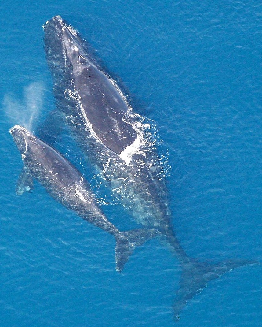
We’ll start with whales, like the Atlantic Right Whale mother and calf shown on the left. Whales almost always give birth to one calf. This birth follows a long gestation period (pregnancy), which ranges from 10 months to up to a year and a half (depending on the type of whale). After her calf is born, a whale mother will nurse her calf for up to two years (again, the period depends on the species). Once that calf grows to be an adult, it can live for up to 70 years.
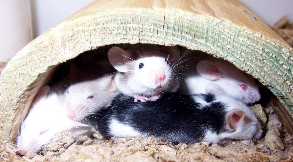
Now let’s think about mice. Mice can live for 12 to 18 months. Their gestation period ranges from about 3 weeks to a month. A litter typically consists of 5 – 6 pups. Nursing lasts for about three weeks. By six weeks of age, a female mouse is sexually mature.
In a previous tutorial about adaptation and natural selection, we explored how a population is selected by the environment for traits that maximize fitness. Fitness involves maximizing the number of one’s descendants. But maximizing one’s descendants doesn’t necessarily mean having a lot of offspring. In some circumstances, fecundity — the ability to produce abundant offspring — is indeed the best evolutionary strategy. In other environments, having very few offspring maximizes fitness.
Among mammals, mice and whales represent the two extremes of selection for traits related to how many offspring are typically born to mothers, and how much energy parents invest in their offspring. Mice are “r-selected.” The “r” refers to selection for reproductive rate. Species that are r-selected live in environments with less predictable resources. They produce more offspring and invest only a little in each one’s survival.
Whales are “K-selected.” The “K” refers to carrying capacity. Species that are K-selected live in more stable, predictable environments. They produce relatively few young, but invest a lot in each one, trying to ensure each offspring’s successful survival.
Based on what you’ve read above, complete the questions below.
[qwiz qrecord_id=”sciencemusicvideosMeister1961-r vs K selection (v2.0)”]
[h]r vs K selection
[i]
[q labels = “top”]Start by completing this table.
| r-selection | K-selection | |
| body size | _____________ | _____________ |
| Life span | _____________ | _____________ |
| Energy investment by parent(s) | _____________ | _____________ |
| number of offspring produced | _____________ | _____________ |
| survivorship curve | _____________ | _____________ |
| Population regulation | _____________ _____________ |
_____________ _____________ |
| Timing of sexual maturation | _____________ | _____________ |
[l]density dependent
[fx] No. Please try again.
[f*] Good!
[l]density independent
[fx] No. Please try again.
[f*] Excellent!
[l]early
[fx] No. Please try again.
[f*] Great!
[l]few
[fx] No, that’s not correct. Please try again.
[f*] Excellent!
[l]high
[fx] No, that’s not correct. Please try again.
[f*] Excellent!
[l]large
[fx] No, that’s not correct. Please try again.
[f*] Correct!
[l]late
[fx] No. Please try again.
[f*] Excellent!
[l]long
[fx] No. Please try again.
[f*] Great!
[l]low
[fx] No. Please try again.
[f*] Excellent!
[l]many
[fx] No. Please try again.
[f*] Excellent!
[l]small
[fx] No, that’s not correct. Please try again.
[f*] Good!
[l]short
[fx] No. Please try again.
[f*] Good!
[l]Type 1
[fx] No. Please try again.
[f*] Great!
[l]Type 3
[fx] No, that’s not correct. Please try again.
[f*] Good!
[q labels = “top”]Let’s think a few of these concepts through in a bit more detail. In an ___________ and/or unpredictable environment, the chance of an organism’s young surviving is very ______. With odds like that, it makes sense to have a lot of ___________, but to invest relatively little in each one, hoping that at least ______ survives.
That’s the strategy taken by _____________ species. In the plant world, it’s exemplified by the dandelion shown on the left. With the seeds randomly distributed by the _________, it makes evolutionary sense to ________ very little in each one. This is typical of species with a _________ survivorship curve.
[l]invest
[fx] No. Please try again.
[f*] Good!
[l]low
[fx] No, that’s not correct. Please try again.
[f*] Excellent!
[l]offspring
[fx] No. Please try again.
[f*] Correct!
[l]one
[fx] No. Please try again.
[f*] Great!
[l]r-selected
[fx] No. Please try again.
[f*] Correct!
[l]Type III
[fx] No, that’s not correct. Please try again.
[f*] Great!
[l]unstable
[fx] No. Please try again.
[f*] Correct!
[l]wind
[fx] No. Please try again.
[f*] Good!
[q labels = “top”]By contrast, imagine an environment that’s predictable and stable. In that type of environment, it’s a _________ bet that there will be food, shelter, and other ___________ required for survival. In that case, it makes evolutionary success to __________ a lot in each young’s survival. In addition, species in this kind of environment will be selected to have a _______ survivorship curve, with most organisms living into ____________. And a big factor behind survivorship will be the ___________ investment that each individual receives.
[l]adulthood
[fx] No, that’s not correct. Please try again.
[f*] Good!
[l]good
[fx] No. Please try again.
[f*] Correct!
[l]invest
[fx] No. Please try again.
[f*] Great!
[l]resources
[fx] No, that’s not correct. Please try again.
[f*] Excellent!
[l]parental
[fx] No, that’s not correct. Please try again.
[f*] Great!
[l]type I
[fx] No. Please try again.
[f*] Good!
[/qwiz]
8. Population Ecology Flashcards
[qdeck qrecord_id=”sciencemusicvideosMeister1961-Population Ecology Flashcards (v2.0)”]
[h]Population Ecology Flashcards
[i]
[q json=”true” yy=”4″ unit=”8.Ecology” dataset_id=”AP_Bio_Flashcards_2022|11b6669b3e510″ question_number=”391″ topic=”8.3-4.Population_Ecology”] Ultimately, only four variables affect the size of any population. What are they?
[a] Population size is a function of births, deaths, immigration, and emigration.
[q json=”true” yy=”4″ unit=”8.Ecology” dataset_id=”AP_Bio_Flashcards_2022|11a5aa85c7910″ question_number=”392″ topic=”8.3-4.Population_Ecology”] What is exponential growth?
[a] Exponential growth is the growth of a population in which the number of individuals added is proportional to the amount already present. As a result, the bigger the population, the bigger the increase.
[q json=”true” dataset_id=”AP_Bio_Flashcards_2022|8bc500335071b” question_number=”393″ unit=”8.Ecology” topic=”8.3-4.Population_Ecology”] Explain the formula for exponential growth.
[a] The formula for exponential growth is change in N/t = rN, where
- N = population size
- t = time
- r= rate of increase
[q json=”true” dataset_id=”AP_Bio_Flashcards_2022|8badb7bc6871b” question_number=”394″ unit=”8.Ecology” topic=”8.3-4.Population_Ecology”] In a graph, what does exponential growth look like?
[a] When exponential growth is plotted (with time as the X-axis and population size as the Y-axis) the result is a J-shaped curve: a slow takeoff followed by an increasingly steep rise in population.
[q json=”true” yy=”4″ unit=”8.Ecology” dataset_id=”AP_Bio_Flashcards_2022|1195837349d10″ question_number=”395″ topic=”8.3-4.Population_Ecology”] In biological systems, when does exponential growth occur?
[a] In any biological system, exponential growth can only happen for a limited period, during which a population has the resources (food, space, etc) that let it grow without constraints. This might happen when an invasive species arrives in a new environment, free from the predators that might have held it in check in its previous environment. It can also happen during the early phases of a bacterial infection, or during a disease outbreak (when a pathogen can spread exponentially).
[q json=”true” yy=”4″ unit=”8.Ecology” dataset_id=”AP_Bio_Flashcards_2022|11886ab067510″ question_number=”396″ topic=”8.3-4.Population_Ecology”] What is biotic potential? How is it represented?
[a] Biotic potential is the maximum rate at which a population can expand. It’s represented by rmax.
[q json=”true” dataset_id=”AP_Bio_Flashcards_2022|1c0f35b12e05″ question_number=”397″ unit=”8.Ecology” topic=”8.3-4.Population_Ecology”] What is carrying capacity?
[a] Carrying capacity (K) is the maximum number of individuals that a particular environment can support.
[q json=”true” yy=”4″ unit=”8.Ecology” dataset_id=”AP_Bio_Flashcards_2022|1178fde1a0d10″ question_number=”398″ topic=”8.3-4.Population_Ecology”] What is the logistic growth model?
[a] The logistic model of population growth shows how a population’s growth rate decreases as it reaches its carrying capacity (E).
[q json=”true” dataset_id=”AP_Bio_Flashcards_2022|8b3769203731b” question_number=”399″ unit=”8.Ecology” topic=”8.3-4.Population_Ecology”] Describe the equation for logistic growth.
[a] The logistic growth model can be represented by the equation N/t = rN (K-N)/K, where
- N = population size
- t = time
- r= rate of increase
- K = carrying capacity
As a population reaches its carrying capacity, there will be increased environmental resistance, as density-dependent limiting factors slow and then stop a population’s growth.
[q json=”true” dataset_id=”AP_Bio_Flashcards_2022|8b0992761e71b” question_number=”400″ unit=”8.Ecology” topic=”8.3-4.Population_Ecology”] When plotted on a graph, what does logistic growth look like?
[a] When logistic growth is plotted (with the X-axis representing time and the Y-axis representing population size), the result is an “S-shaped” or “sigmoid” curve. The curve initially looks like an exponential growth curve (a J-curve) with a slow takeoff followed by a rapid rise (A and B). But as N approaches carrying capacity, the amount of increase slows (C) and then drops to zero (D) as the population stabilizes at its carrying capacity (E).
[q json=”true” yy=”4″ unit=”8.Ecology” dataset_id=”AP_Bio_Flashcards_2022|1139665cdd910″ question_number=”401″ topic=”8.3-4.Population_Ecology”] In relationship to population growth, what are limiting factors?
[a] Limiting factors prevent a population from increasing at its biotic potential, and cause a population’s size to stabilize at or below the environment’s carrying capacity.
[q json=”true” dataset_id=”AP_Bio_Flashcards_2022|1a2d4013d205″ question_number=”402″ unit=”8.Ecology” topic=”8.3-4.Population_Ecology”] Define and describe density-dependent limiting factors.
[a] Density-dependent limiting factors intensify as the density of individuals within a population increases. These factors can be extrinsic (coming from outside the growing population) or intrinsic (from within the population).
Extrinsic factors include predation pressure, parasitism, and competition for increasingly scarce resources. Intrinsic factors can include the stress that’s induced by increased crowding and competition, lowering the birth rate. Territoriality can similarly decrease a population’s ability to expand beyond a certain density.
[q json=”true” dataset_id=”AP_Bio_Flashcards_2022|198a44d37a05″ question_number=”403″ unit=”8.Ecology” topic=”8.3-4.Population_Ecology”] Define and describe density-independent limiting factors.
[a] Density-independent limiting factors are those that are unrelated to a population’s size (symbolized by N). For example, hurricanes, floods, or earthquakes can all cause significant death in a population, lowering population size, regardless of that population’s density.
[q json=”true” yy=”4″ unit=”8.Ecology” dataset_id=”AP_Bio_Flashcards_2022|1125c13889d10″ question_number=”404″ topic=”8.3-4.Population_Ecology”] When a population reaches its carrying capacity, the result might be stable oscillation around carrying capacity. Explain.
[a] In this scenario, the population overshoots the carrying capacity (E), lowering the available resources. This causes the population to decline (F). As the resource base recovers, the population resumes its growth until it again overshoots the carrying capacity (G), repeating the cycle.
[q json=”true” dataset_id=”AP_Bio_Flashcards_2022|22226ae15b55a5″ question_number=”405″ unit=”8.Ecology” topic=”8.3-4.Population_Ecology”] Sometimes, a population overshoots carrying capacity, which is followed by a catastrophic population decline. Explain.
[a] An overshoot (2) is where the population exceeds the environment’s carrying capacity. If this causes a significant depletion in environmental resources from which the environment can’t recover, then the population that caused the depletion, if it can survive at all, will do so at significantly reduced numbers.
[x][restart]
[/qdeck]
9. Population Ecology: Summative Quiz
This quiz will test you on everything in this module on population ecology.
[qwiz random = “true” qrecord_id=”sciencemusicvideosMeister1961-Population Ecology: Summative Quiz (v2.0)”]
[h]Population Ecology: Summative Quiz
[i]
[q] In the diagram below, which letter represents the carrying capacity?
[textentry single_char=”true”]
[c]IE U=[Qq]
[f]IEV4Y2VsbGVudC4gJiM4MjIwO0UmIzgyMjE7IHJlcHJlc2VudHMgY2FycnlpbmcgY2FwYWNpdHk=[Qq]
[c]IEVudGVyIHdvcmQ=[Qq]
[f]IE5vLCB0aGF0JiM4MjE3O3Mgbm90IGNvcnJlY3Qu[Qq]
[c]ICo=[Qq]
[f]IE5vLiBZb3UmIzgyMTc7cmUgbG9va2luZyBmb3IgYSBsaW5lIHRoYXQgcmVwcmVzZW50cyB0aGUgbWF4aW11bSBwb3B1bGF0aW9uIHRoYXQgdGhpcyBhcmVhIG9yIGVudmlyb25tZW50IGNvdWxkIHN1cHBvcnQu[Qq]
[q] In the diagram below, which letter represents the point at which the population has reached the environment’s carrying capacity?
[textentry single_char=”true”]
[c]IE Q=[Qq]
[f]IEF3ZXNvbWUuICYjODIyMDtEJiM4MjIxOyBpcyB0aGUgcG9pbnQgYXQgd2hpY2ggdGhpcyBwb3B1bGF0aW9uIGhhcyByZWFjaGVkIGl0cyBjYXJyeWluZyBjYXBhY2l0eS4=[Qq]
[c]IEVudGVyIHdvcmQ=[Qq]
[f]IFNvcnJ5LCB0aGF0JiM4MjE3O3Mgbm90IGNvcnJlY3Qu[Qq]
[c]ICo=[Qq]
[f]IE5vLiBMb29rIGZvciB0aGUgcG9pbnQgaW4gdGhlIGJsYWNrIGxpbmUgd2hlcmUgdGhlIHNsb3BlIGlzIHRoZSBzdGVlcGVzdC4=[Qq]
[q] The kind of population growth shown below is [hangman] growth. It only occurs when there are no [hangman] factors at work.
[c]IGV4cG9uZW50aWFs[Qq]
[f]IEdyZWF0IQ==[Qq]
[c]IGxpbWl0aW5n[Qq]
[f]IEV4Y2VsbGVudCE=[Qq]
[q] The kind of population growth shown below is called [hangman] growth. In this growth model, a population’s growth slows as it reaches the environments’ [hangman] [hangman].
[c]IGxvZ2lzdGlj[Qq]
[f]IEdvb2Qh[Qq]
[c]IGNhcnJ5aW5n[Qq]
[f]IENvcnJlY3Qh[Qq]
[c]IGNhcGFjaXR5[Qq]
[f]IENvcnJlY3Qh[Qq]
[q] Environmental factors such as fires, floods, landslides, and volcanic eruptions would all be classified as [hangman] [hangman] limiting factors
[c]IGRlbnNpdHk=[Qq]
[f]IEdvb2Qh[Qq]
[c]IGluZGVwZW5kZW50[Qq]
[f]IEdvb2Qh[Qq]
[q] Limiting factors such as competition, parasitism, predation, and waste accumulation are all classified as [hangman] factors because they come from outside of the population itself.
[c]IGV4dHJpbnNpYw==[Qq]
[f]IENvcnJlY3Qh[Qq]
[q] In the diagram below, which number or letter refers to the “overshoot.”
[textentry single_char=”true”]
[c]ID I=[Qq]
[f]IE5pY2Ugam9iLiBUaGUgb3ZlcnNob290IGlzIHJlcHJlc2VudGVkIGJ5ICYjODIyMDsyLiYjODIyMTs=[Qq]
[c]IEVudGVyIHdvcmQ=[Qq]
[f]IE5vLg==[Qq]
[c]ICo=[Qq]
[f]IE5vLiBUaGUgb3ZlcnNob290IGlzIHRoZSBwb2ludCB3aGVyZSB0aGUgcG9wdWxhdGlvbiBncm93cyBiZXlvbmQgdGhlIGVudmlyb25tZW50JiM4MjE3O3MgY2FycnlpbmcgY2FwYWNpdHkuIFdoZXJlIHdvdWxkIHRoYXQgYmU/[Qq]
[q] The graph below shows the results of a computer model of the interaction between a population of predators and a population of prey. Which number represents the predator?
[textentry single_char=”true”]
[c]ID I=[Qq]
[f]IEF3ZXNvbWUuIFRoZSBwcmVkYXRvciYjODIxNztzIHBvcHVsYXRpb24gaXMgcmVwcmVzZW50ZWQgYnkgJiM4MjIwOzIuJiM4MjIxOw==[Qq]
[c]IEVudGVyIHdvcmQ=[Qq]
[f]IE5vLCB0aGF0JiM4MjE3O3Mgbm90IGNvcnJlY3Qu[Qq]
[c]ICo=[Qq]
[f]IE5vLiBKdXN0IHRoaW5rIGFib3V0IHdoYXQgeW91IGtub3cgYWJvdXQgdGhlIHJlbGF0aW9uc2hpcCBiZXR3ZWVuIHByZWRhdG9ycyBhbmQgcHJleSBpbiBuYXR1cmUuIFRoaW5rIHRocm91Z2ggdGhlIGJsYW5rcyBpbiB0aGlzIGhpbnQsIGFuZCB5b3UmIzgyMTc7bGwgaGF2ZSB0aGUgYW5zd2VyOiB0aGVyZSBhcmUgYWx3YXlzIGZld2VyIF9fX19fX19fXyB0aGFuIHByZXku[Qq]
[q multiple_choice=”true”] A species that is a K-strategist is most likely to have a
[c]IHNob3J0IGxpZmUgc3Bhbi4=[Qq]
[f]IE5vLiA=Sy0=c3RyYXRlZ2lzdA==cw==IHRlbmQgdG8gYmUgbG9uZy1saXZlZC4=[Qq]
[c]IHNtYWxsIGluIHNpemUu[Qq]
[f]IE5vLiBXaXRoaW4gdGhlaXIgY2xhZGUsIA==Sy0=c3RyYXRlZ2lzdA==cw==IHRlbmQgdG8gYmUgbGFyZ2Uu[Qq]
[c]IGxhcmdlIG51bWJlciBvZiBvZmZzcHJpbmcu[Qq]
[f]IE5vLiA=Sy0=c3RyYXRlZ2lzdA==cw==IHRlbmQgdG8gaGF2ZSBmZXcgb2Zmc3ByaW5nLg==[Qq]
[c]IGxvbmcgcGVyaW9kIG9m IHBhcmVudGFsIGNhcmUu[Qq]
[f]IFdheSB0byBnby4gSy0=c3RyYXRlZ2lzdA==cw==IHRlbmQgdG8gaGF2ZSBmZXcgb2Zmc3ByaW5nIGFuZCBwcm92aWRlIHRoZW0gd2l0aCBsb3RzIG9mIGNhcmUu[Qq]
[q]Limiting factors such as disease from parasites, increased predation, and food scarcity is all density [hangman]. As this population continues to grow within the same area, these factors will become more [hangman].
[c]ZGVwZW5kZW50[Qq]
[c]aW50ZW5zZQ==[Qq]
[/qwiz]
What’s Next?
Proceed to Topic 8.5, Community Ecology, Part 1: Species Interactions (the next tutorial in AP Bio Unit 8, Ecology).